Well I’m here. My trip ended up being 27 hours and it was great to get here and sleep and wake up to a delicious telescope breakfast:
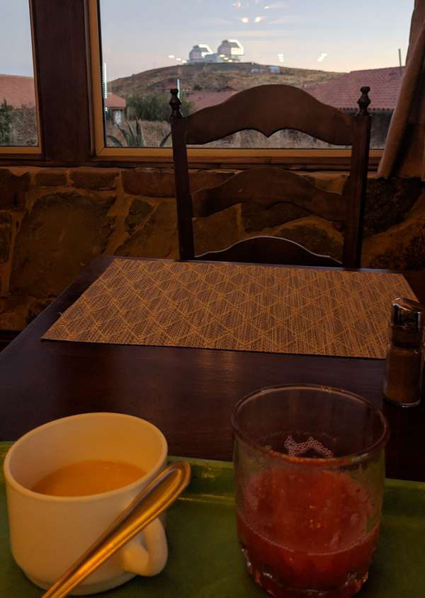
[Image description: Photo of 2 telescope domes on the top of the mountain, with a breakfast chair and some half-drinken tea and juice in the foreground]
I found this fine literature in the desk drawer in my room, left from a previous inhabitant:
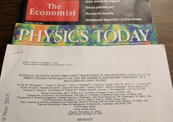
[Image description: The fine literature includes The Economist, Physics Today, and an ApJ paper by the author]
Today we worked hard on cooling and code. Clio code, AO code, DigiPort code. The mountain internet was down for about 4 hours. Laird arrived safely and the mystery guest got stranded in Santiago and will be here hopefully tomorrow.
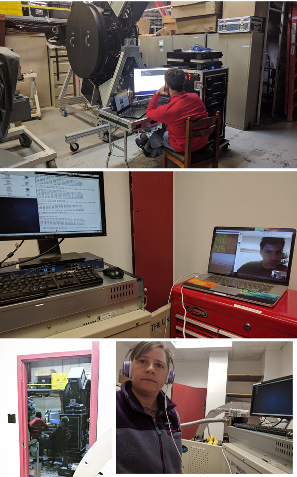
[Image description: A collage of Jared working on AO code, Paul Skyping with Katie on Clio code, Jared and Laird by the NAS, and Katie with Clio]
I did manage to get Clio down to almost 77 K in one day! Clio drank his liquid nitrogen very well today.
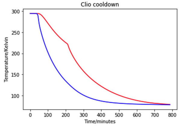
[Image description: A line plot with a red and a blue curve, showing the temperature dropping. The x axis is time in minutes and the y axis is temperature in Kelvin. Both dewars start flat at the ambient temperature, around 295 K. The curves drop exponentially, but the outer dewar drops at a faster rate than the inner dewar. There is a point of inflection in the inner dewar curve, at the point where the outer dewar got below 150 K. This is where I started filling the inner dewar too; before that it was only cooling passively. Both curves asymptote to around the temperature of liquid nitrogen, 77 K.]
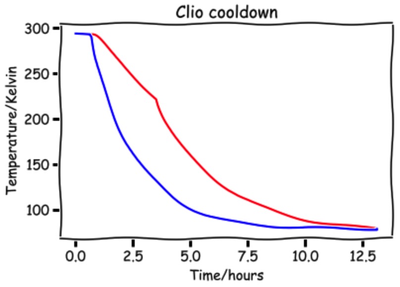
[Image description: The same line plot as above, only I decided to put the x-axis in hours, and I used the “XKCD” style in MatPlotLib so that it looks like my plot was hand-drawn by Randall Munroe]
And we saw a herd of 5 guanacos running along the hillside as we were heading back up after lunch:
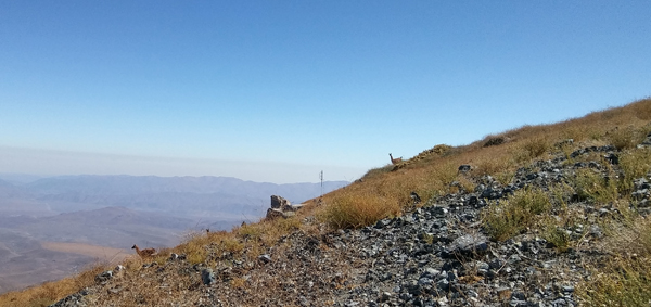
[Image description: Guanacos on a hillside in Chile. They are kind of like llamas. They are pretty far away in the picture.]
Today’s song:
[Song/image description: “Come” by Jain]
[Song/image description: cover of “Come” by Esteban and Laura]